Convolutional Neural Network
[Download this notebook](09 - Convolutional Neural Network.ipynb)
This week we are looking at convolutional neural networks. Convolutional neural networks (CNNs) are used primarily, but not exclusively, for image recognition.
Unlike the neural networks we have seen so far, CNNs can read images as a matrix. This means that local context is not lost by flattening the image.
Otavio Good. 2017 “A Visual and Intuitive Understanding of Deep Learning” O’Reilly AI Conference
import torch
from torch import nn
import pandas as pd
import numpy as np
from matplotlib import pyplot as plt
from torch.utils import data

def min_max(x):
    return (x - np.min(x)) / (np.max(x) - np.min(x))
First, reload the training data and convert it to a tensor. In total there are 60,000 images with 784 pixels + a column for the labels of the images.
train_data = pd.read_csv('https://uni-muenster.sciebo.de/s/xSU1IKM6ui4WKAV/download', delimiter=',', header=None).values

train_x = torch.tensor(min_max(train_data[:,1:]), dtype=torch.float32)
train_y = torch.tensor(train_data[:,0], dtype=torch.long)

print(train_x.shape, train_y.shape)
So far, we have always input images as 1D vectors to our neural network. But this time we want to use the 2D structure. For this we have to make a matrix of size 28 x 28 out of a vector of length 784.
For this we can use the function vector.view(28,28).
train_x[0,:].view(28,28).shape
We can look at this picture, but we can’t see much.
train_x[0,:].view(28,28)
But with matplotlib we can represent arrays as an image. Here cmap = "gray" specifies that we want our color spectrum to be black and white only.
plt.imshow(train_x[0,:].view(28,28), cmap= "gray")
We only have one image in the correct format so far, to do this for all images we can also use .view(). The tensor we created before had the format (height,width). To be able to convert all images, we need to add an additional dimension to the tensor. The new tensor should have the following dimensions: (number of images, height, width). So we have a total of three dimensions.
However, PyTorch would throw a wrench in our plans here. Because PyTorch can work with black and white (b/w) as well as with colored images. In PyTorch, colored images are represented by three matrices. One for red, one for green and one for blue. These are also called channels. A colored image would have the dimensions (3, height, width) in PyTorch. So the dimension we just used for number of images is occupied by the number of channels.

PyTorch expects this “channel dimension” also for b/w images.
Therefore we represent a b/w image as follows: (1, height, width).
It follows that all images from the MNIST dataset must match this format: (number of images, 1, height, width). So in total our input tensor has 4 dimensions.
Convert train_x to this format.
train_x = train_x.view(_____,1,____,____)
train_x.shape
train_x = train_x.view(60000,1,28,28)
You have now converted all images to the format (1,28,28).
You can still display images with plt.imshow.
Notice how the tensor is now indexed. [0,0,:,:]. We select the first image and also the first and only channel. We also select the entire height and width to display the image completely.
plt.imshow(train_x[0,0,:,:], cmap= "gray")
Like in the last notebook you can use a DataLoader. For this you have to create a PyTorch dataset first. With next(iter()) you can output the first minibatch of the DataLoader.
torch_train = data.TensorDataset(_____, ____)
train_loader = data.DataLoader(______, batch_size=32)

batch_x, batch_y =next(iter(train_loader))
print(batch_x.shape, batch_y.shape)
torch_train = data.TensorDataset(train_x,train_y)
train_loader = data.DataLoader(torch_train, batch_size=32)

batch_x, batch_y =next(iter(train_loader))
print(batch_x.shape, batch_y.shape)
As you can see, the batch_x has the dimensions [32, 1, 28, 28]. So 32 images, the size of our batch, 1 channel, 28 pixels in height and 28 in width.
Create CNNs in PyTorch.
So far we have our data in the right format, now it is time to create a CNN in PyTorch. Just as there are nn.Linear layers in PyTorch, there are also Convolutional Layers in the nn module.
nn.Conv2d() is one such layer. Before we use it, we briefly discuss the most important parameters.
in_channelsthe number of channels the image has before convolution .out_channelshow many channels the image should have after convolution. Or how many filters we run over the image.kernel_sizehow big the kernel is, so the height/width in pixels.
conv1 = nn.Conv2d(in_channels=1, out_channels=3, kernel_size=3)
out = conv1(batch_x)
out.shape
As you can see, the size of the minibatch has changed. We still have 32 images, but as indicated, we now have 3 channels. The height and width of our image have also changed. We have lost 2 pixels per dimension. This is due to the way the convolution works.
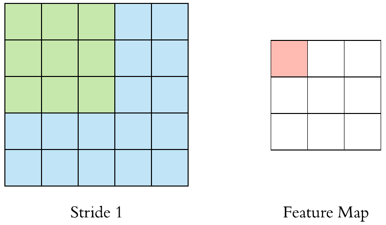
Here is an example of why a kernel size of 3 makes our output image two pixels smaller. On the left is the input image and on the right is the output image. Since we can’t push the kernel over the edge of the image, we “lose” the outer edge of the image.
To prevent this information from being lost, we can pad the image. This way we enlarge the image, for example with pixels that have the value zero.
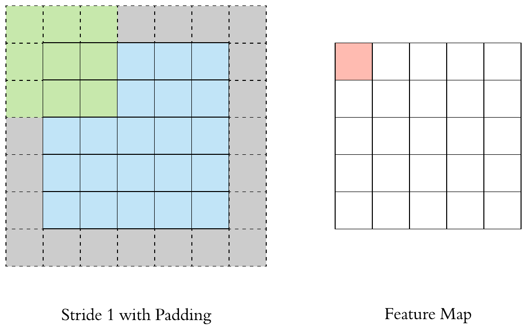
By padding, the kernel can be pushed once over the entire image.
We can also specify the width of the padding as a parameter in Conv2d.
conv1 = nn.Conv2d(in_channels=1, out_channels=3, kernel_size=3, padding =1)
out = conv1(batch_x)
out.shape
Due to the padding the image does not shrink anymore. Since we now have 3 channels, we can still display the image using plt.imshow. To do this, we need to select an image from the minibatch and use the detach() command to remove the gradients stored by autograd.
An image like this can only be used as an example to illustrate the transformation. The actual colors and intensities are irrelevant here, since these are arbitrarily set by the network.
plt.imshow(min_max(out.detach().numpy()[0].transpose((1, 2, 0))))
You can still see a 5, but this time in color. As described above, the colors can not be used for interpretation. They are only used to show the diversification of the input.
The second new layer you will use today is nn.MaxPool2d().
This layer is called the Pooling layer.
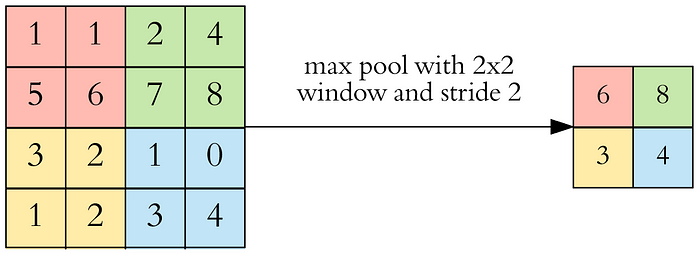
Pooling layers leads to a deliberate reduction in image size deeper in the network. This means that fewer parameters (weights) are needed, which results in our networks training faster. When you look at an image (larger than 28 x 28 pixels), you don’t recognize each pixel individually, but pixels in a certain proximity merge together. Pooling works in a similar way. Here, multiple pixels are combined using the maximum value. Fewer parameters also mean a lower probability of overfitting.
The most commonly used pooling layer is the max pooling layer. Here the largest value in the region is chosen as the new value for the output. There are, of course, a variety of other pooling layers.
In addition to the kernel size, the size of the square we want to pool, this time we also specify the stride. The stride determines by how many pixels we move the pooling kernel.

Here is a website with which you can visualize the effect of different parameters on the convolution.
pool1 = nn.MaxPool2d(kernel_size = 2, stride = 2)
You can now use the output of the 2DConv (out) as input for the pooling layers.
out2 = pool1(____)
out2.shape
out2 = pool1(out)
Since the number of channels has not changed, we can still visualize this image. We can see that the image has shrunk, yet you can still see the 5.
plt.imshow(min_max(out2.detach().numpy()[0].transpose((1, 2, 0))))
With nn.Sequential you can also write several convolution/pooling layers in a row. Important, we also need a nonlinear activation function again, this is normally inserted after the convolution.
Fill in the missing code:
cnn = nn.Sequential(nn.Conv2d(in_channels=_, out_channels=3, kernel_size=3, padding =1),
                   nn.ReLU(),
                   nn.MaxPool2d(kernel_size = 2,stride = 2),
                   nn.Conv2d(in_channels= _ , out_channels=6, kernel_size=3, padding =1),
                   nn.______,
                   nn.MaxPool2d(kernel_size = 2,stride = 2))
cnn = nn.Sequential(nn.Conv2d(in_channels=1, out_channels=3, kernel_size=3, padding =1),
                   nn.ReLU(),
                   nn.MaxPool2d(kernel_size = 2,stride = 2),
                   nn.Conv2d(in_channels= 3 , out_channels=6, kernel_size=3, padding =1),
                   nn.ReLU(),
                   nn.MaxPool2d(kernel_size = 2,stride = 2))
Now we can pass batch_x through the network.
cnn(batch_x).shape
However, this output is not yet suitable for predictions. For this, we have to feed the images back into a conventional neural network. However, these only accept inputs in the form of vectors. So we convert each image back into a vector.
The output tensor has the shape [32, 6, 7, 7] and should become a tensor of size [32, 6 x 7 x 7] = [32, 294].
For this we can use the layer nn.Flatten(starting_dim). Here we only have to define the parameter starting_dim. This determines from which dimension we merge the dimensions. Since we want a separate vector for each image, we use starting_dim = 1. With cnn.add_module() we can add additional layers to our network.
cnn.add_module("flatten",nn.Flatten(1))
cnn(batch_x).shape
The size of the batch is now (32,294). 32 is still the number of images in the batch (dimension 0), but our second dimension is now 294. This means that each image in the batch has a vector associated with it. Now we can also add a traditional linear layer. However, before the layer nn.Linear we add an additional BatchNorm and a dropout layer.
cnn.add_module("bn", nn.BatchNorm1d(____))
cnn.add_module("dp", nn._________(0.2))
cnn.add_module("fc", nn.Linear(____,___))
cnn.add_module("bn", nn.BatchNorm1d(294))
cnn.add_module("dp", nn.Dropout(0.2))
cnn.add_module("fc", nn.Linear(294,10))
Now you can set the loss function and optimizer. Using PyTorch’s loaders and the nn module, you can copy the same for-loop from last notebook without change.
loss_function = nn.CrossEntropyLoss()
update =  torch.optim.Adam(_____________, lr =0.001)
loss_funktion = nn.CrossEntropyLoss()
update =  torch.optim.Adam(cnn.parameters(), lr =0.001)
EPOCHS = 2
for i in range(EPOCHS):
    loss_list = []
    cnn.train()
    for minibatch in train_loader:
        images, labels = minibatch

        update.zero_grad()
        output = cnn(images)
        loss   = loss_function(output, labels)
        loss.backward()
        loss_list.append(loss.item())
        update.step()
    cnn.eval()
    output = cnn(train_x)
    train_acc=((output.max(dim=1)[1]==train_y).sum()/float(output.shape[0])).item()
    print(
        "Training Loss: %.2f Training Accuracy: %.2f"
        % (np.mean(loss_list), train_acc)
    )
Last, we evaluate the network on the test dataset.
test_data = pd.read_csv('https://uni-muenster.sciebo.de/s/fByBt5wd24chROg/download', delimiter=',', header = None).values
test_x = torch.tensor(min_max(test_data[:,1:]), dtype=torch.float32)
test_y = torch.tensor(test_data[:,0], dtype=torch.long)
test_x = test_x.reshape(test_x.shape[0],1,28,28)
print(test_x.shape, test_y.shape)
output = cnn(test_x)
acc=((output.max(dim=1)[1]==test_y).sum()/float(output.shape[0])).item()
acc
Practice Exercise
Again we use the toxicity data for the exercise task. However, this time the molecules are not in SMILES format, but the structures are stored as an image. You will again predict the toxicity, but this time based on the image.
In fact, this has already been attempted.
The images consist of 64 x 64 pixels. You will see that this is barely sufficient to see the molecular structure. However, we are bound to the memory space provided by the university.
And a higher resolution does not change the underlying task.
Restart the kernel before beginning the exercise!
import numpy as np
import torch
from torch import nn
from torch.utils import data
from matplotlib import pyplot as plt
import pandas as pd
from sklearn.model_selection import train_test_split
import torchvision.transforms as T
def min_max(x):
    return (x - np.min(x)) / (np.max(x) - np.min(x))
First, divide the data into training set and test set. Important: the last column contains the information about the toxicity. So this is our variable to predict.
mol_img_data = torch.tensor(pd.read_csv('https://uni-muenster.sciebo.de/s/oW8odaLJCgqycS3/download',
                                        delimiter = ',',
                                        header = None).values,
                            dtype = torch.float32)

train, test=train_test_split(_______________,______________,_________, random_state=1234)

train_x = train[______]
train_y = train[______]
test_x = test[______]
test_y = test[______]


print(train_x.shape, train_y.shape)
This is how pixelated the images look:
plt.imshow(train_x[10,:].view(64,64), cmap= "gray")
Next, convert the test and training set. Remember that the dimensions should look like this. Number of Images, Number of Channels, Height, Width.
train_x = train_x.view(__________________________)
test_x = test_x.view(___________________________)
torch_train = data.TensorDataset(______________________)
train_loader = data.DataLoader(__________________, batch_size=32)

batch_x, batch_y =next(iter(train_loader))
print(batch_x.shape, batch_y.shape)
If you have done everything right so far, batch_x should have the dimensions [32, 1, 64, 64] and batch_y should have the dimensions [32]. Add at least 2 more convolution layers to the network. Make sure you also use pooling layers and non-linear activation functions.
cnn = nn.Sequential(nn.Conv2d(in_channels= , out_channels , kernel_size , padding ),


                   )
cnn(batch_x).shape
Now add a flatten layer. From which dimension do we start to add the values together?
cnn.add_module("flatten",nn.Flatten(_))
cnn(batch_x).shape
At last add a BatchNorm, Dropout and Linear layer. Make sure you use the correct input/output dimensions.
cnn.add_module("bn", _______________)
cnn.add_module("dp", _______________)
cnn.add_module("fc", _______________)
cnn(batch_x).shape
The shape should now be [32, 1]. Fill in the rest of the training loop.
loss_funktion = ________________________
update =  torch.optim.Adam(_______________, lr =0.0003)
EPOCHS = 30


for i in range(EPOCHS):
    loss_list = []

    ___.train()
    for minibatch in train_loader:
        images, labels = minibatch
        ________.zero_grad()
        output = cnn(_______)
        loss   = loss_function(output.squeeze(), labels)
        loss.backward()
        loss_list.append(loss.item())
        update.step()
    ___.eval()

    # Training Evaluation
    output = cnn(train_x)
    train_acc = torch.sum((output>0).squeeze().int() == train_y)/train_y.shape[0]
    # Test Evaluation
    output = cnn(test_x)
    loss   = loss_function(output.squeeze(), test_y)
    test_acc = torch.sum((output>0).squeeze().int() == test_y)/test_y.shape[0]

    print(
        "Training Loss: %.2f Training Accuracy: %.2f | Test Loss: %.2f  Test Accuracy: %.2f"
        % (np.mean(loss_list), train_acc, loss.item(),test_acc )
    )
As you can see, this works only moderately. It definitely works better with fingerprints. Generally, it is more difficult to train CNNs than simpler neural networks. Furthermore, drawing molecules is very inefficient compared to calculation of SMILES or fingerprints/descriptors.
In our case, one could argue that our model could also learn better if we had larger and more colorful images. This is probably true. But even in the above paper, CNNs simply could not beat networks with fingerprints. It can be said that images are not an adequate representation of molecules. At least not for machine learning.
This is not to say that it cannot be useful to train CNNs on images of molecules. For example, networks that recognize structures and output the appropriate SMILES. This can be used to quickly search patents and chemical publications.
For example here: https://jcheminf.biomedcentral.com/articles/10.1186/s13321-021-00538-8